#Import Librariesimport numpy as npimport geopandas as gpdimport rioxarray as rioxrimport matplotlib.pyplot as pltfrom shapely.geometry import Polygon# used to access STAC catalogsfrom pystac_client import Client# used to sign items from the MPC STAC catalogimport planetary_computer# ----- other libraries for nice ouputsfrom IPython.display import Image
Access
We use the Client function from the pystac_client package to access the catalog:
The modifier parameter is needed to access the data in the MPC catalog.
Exploration
Let’s check out some of the catalog’s metadata:
# metadata from the catalog#print('ID:', catalog.id)print('Title:', catalog.title)print('Description:', catalog.description)
Title: Microsoft Planetary Computer STAC API
Description: Searchable spatiotemporal metadata describing Earth science datasets hosted by the Microsoft Planetary Computer
We can access its collections by using the get_collections() method:
catalog.get_collections()
<generator object Client.get_collections at 0x72f428c48f20>
Notice the output of get_collections() is a generator. This is a special kind of lazy object in Python over which you can loop over like a list.
Unlike a list, the items in a generator do not exist in memory until you explicitely iterate over them or convert them to a list. Let’s try getting the collections from the catalog again:
# get collections and print their namescollections =list(catalog.get_collections())print('Number of collections:', len(collections))print("Collections IDs:")for collection in collections:print('-', collection.id)
description: The [National Agriculture Imagery Program](https://www.fsa.usda.gov/programs-and-services/aerial-photography/imagery-programs/naip-imagery/) (NAIP) provides U.S.-wide, high-resolution aerial imagery, with four spectral bands (R, G, B, IR). NAIP is administered by the [Aerial Field Photography Office](https://www.fsa.usda.gov/programs-and-services/aerial-photography/) (AFPO) within the [US Department of Agriculture](https://www.usda.gov/) (USDA). Data are captured at least once every three years for each state. This dataset represents NAIP data from 2010-present, in [cloud-optimized GeoTIFF](https://www.cogeo.org/) format.
We can narrow the search withing the catalog by specifying a time range, an area of interest, and the collection name. The simplest ways to define the area of interest to look for data in the catalog are:
a GeoJSON-type dictionary with the coordinates of the bounding box,
as a list [xmin, ymin, xmax, ymax] with the coordinate values defining the four corners of the bounding box.
In this lesson we will look for the NAIP scenes over Santa Barbara from 2018 to 2020. We’ll use the GeoJSON method to define the area of interest:
#Checksearch# To get the items found in the search (or check if there were any matches in the search) we use the item_collection() method:items = search.item_collection()
Item
Lets get the first item in the list
#get first itemitem = items[0]type(item)
pystac.item.Item
Remember the STAC item is the core object in the catalog and. The item does not contain the data itself, but rather metadata about and links to access the actual data (assets). Some of the metadata:
# print item id and propertiesprint('id:' , item.id)item.properties
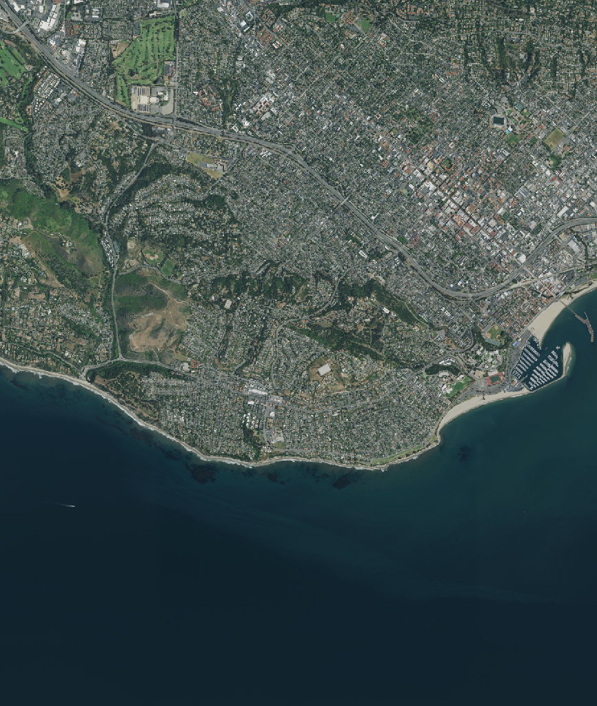
Notice each asset has an href, which is a link to the asset object (i.e. the data). For example, we can use the URL for the rendered preview asset to plot it:
The raster data in our current item is in the image asset. Again, we access this data via its URL. This time, we open it using rioxr.open_rasterio() directly:
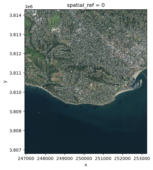
Notice this raster has four bands. So we cannot use the .plot.imshow() method directly (as this function only works when we have three bands). Thus we need select the bands we want to plot (RGB) before plotting:
# plot raster with correct ratiosize =6# height in in of plot heightaspect = sb.rio.width / sb.rio.height # select R,G,B bands and plotsb.sel(band=[1,2,3]).plot.imshow(size=size, aspect=aspect)
<matplotlib.image.AxesImage at 0x72f3a2644ad0>
Exercise:
The ‘cop-dem-glo-90’ collection contains the Copernicus DEM at 90m resolution (the data we previously used for the Grand Canyon).
Reuse the bbox for Santa Barbara to look for items in this collection.
Get the first item in the search and check its assets.
Check the item’s rendered preview asset by clicking on it’s URL.
Open the item’s data using rioxarray.
#Reuse the bbox for Santa Barbara to look for items in this collection.#Catalog Search:search_1 = catalog.search( collections = ['cop-dem-glo-90'], intersects = bbox)
#Check the collectionitems_1 = search_1.item_collection()
#Get the first item in the search.C_DEM = items_1[0]#check its assetsC_DEM.assets